De Bruijn graph alignment should also be useful for exploring concepts in transcriptomics/mRNAseq expression. As with variant calling graphalign can also be used to avoid the mapping step in quantification; and, again, as with the variant calling approach, we can do so by aligning our reference sequences to the graph rather than the reads to the reference sequences.

The basic concept here is that you build a (non-abundance-normalized) De Bruijn graph from the reads, and then align transcripts or genomic regions to the graph and get the k-mer counts across the alignment. This is nice because it gives you a few options for dealing with multimapping issues as well as variation across the reference. You can also make use of the variant calling code to account for certain types of genomic/transcriptomic variation and potentially address allelic bias issues.

Given the existence of Sailfish/Salmon and the recent posting of Kallisto, I don't want to be disingenuous and pretend that this is any way a novel idea! It's been clear for a long time that using De Bruijn graphs in RNAseq quantification is a worthwhile idea. Also, whenever someone uses k-mers to do something in bioinformatics, there's an overlap with De Bruijn graph concepts (...pun intended).

What we like about the graphalign code in connection with transcriptomics is that it makes a surprisingly wide array of things easy to do. By eliminating or at least downgrading the "noisiness" of queries into graphs, we can ask all sorts of questions, quickly, about read counts, graph structure, isoforms, etc. Moreover, by building the graph with error corrected reads, the counts should in theory become more accurate. (Note that this does have the potential for biasing against low-abundance isoforms because low-coverage reads can't be error corrected.)

For one simple example of the possibilities, let's compare mapping counts (bowtie2) against transcript graph counts from the graph (khmer) for a small subset of a mouse mRNAseq dataset. We measure transcript graph counts here by walking along the transcript in the graph and averaging over k-mer counts along the path. This is implicitly a multimapping approach; to get results comparable to bowtie2's default parameters (which random-map), we divide out the number of transcripts in which each k-mer appears (see count-median-norm.py, 'counts' vs 'counts2').

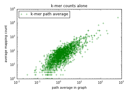
Figure 1: Dumb k-mer counting (x axis) vs dumb mapping (y axis)

This graph shows some obvious basic level of correlation, but it's not great. What happens if we use corrected mRNAseq reads (built using graphalign)?

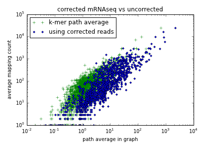
Figure 2: Dumb k-mer counting on error corrected reads (x axis) vs dumb mapping (y axis)

This looks better - the correlation is about the same, but when we inspect individual counts, they have moved further to the right, indicating (hopefully) greater sensitivity. This is to be expected - error correction is collapsing k-mers onto the paths we're traversing, increasing the abundance of each path on average.

What happens if we now align the transcripts to the graph built from the error corrected reads?

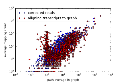
Figure 2: Graphalign path counting on error corrected reads (x axis) vs dumb mapping (y axis)

Again, we see mildly greater sensitivity, due to "correcting" transcripts that may differ only by a base or two. But we also see increased counts above the main correlation, especially above the branch of counts at x = 0 (poor graph coverage) but with high mapping coverage - what gives? Inspection reveals that these are reads with high mapping coverage but little to no graph alignment. Essentially, the graph alignment is getting trapped in a local region. There are at least two overlapping reasons for this -- first, we're using the single seed/local alignment approach (see error correction) rather than the more generous multiseed alignment, and so if the starting point for graph alignment is poorly chosen, we get trapped into a short alignment. Second, in all of these cases, the transcript isn't completely covered by reads, a common occurrence due to both low coverage data as well as incomplete transcriptomes.

In this specific case, the effect is largely due to low coverage; if you drop the coverage further, it's even more exacerbated.

Two side notes here -- first, graphalign will align to low coverage (untrusted) regions of the graph if it has to, although the algorithm will pick trusted k-mers when it can. As such it avoids the common assembler problem of only recovering high abundance paths.

And second, no one should use this code for counting. This is not even a proof of concept, but rather an attempt to see how well mapping and graph counting fit with an intentionally simplistic approach.