tl;dr? Compare and cluster two collections of 1000+ metagenome-assembled genomes in a few minutes with sourmash!
A week ago, someone e-mailed me with an interesting question: how can we compare two collections of genome bins with sourmash?
Why would you want to do this? Well, there's lots of reasons! The main one that caught my attention is comparing genomes extracted from metagenomes via two different binning procedures - that's where I started almost two years ago, with two sets of bins extracted from the Tara ocean data. You might also want to merge bins that were similar to produce a (hopefully) more complete bin, or you could intersect bins that were similar to produce a consensus bin that might be higher quality, or you could identify bins that were in one collection and not in the other, to round out your collection.
I'm assuming this is done by lots of workflows - I note, for example, that the metaWRAP workflow includes a 'bin refinement' step that must do something like this.
I (ahem) haven't really read up on what others do, because I was mostly interested in hacking something together myself. So here goes :).
How do you compare two collections of bins??
There are a few different strategies. My previous attempts were --
-
comparing two directories in bulk, focusing on summary statistics;
-
reclassifying each bin set with the taxonomy from the other bin set
In both cases, my conclusions ended with "wow, there are some real differences here" but I never dug deeply into what was going on in detail.
This time, though, I had a bit more experience under my belt and I realized that a fairly simple thing to do would be to cluster all of the bins together while tracking the origin of each bin, and then deconvolving the clusters so that you could dig into each cluster at arbitrary detail.
The basic strategy
-
Load in two lists of sourmash signatures.
-
Compare them all.
-
Perform some kind of clustering on the all-by-all comparison.
-
Output clusters.
Conveniently, I had already implemented the key bits in a Jupyter notebook about a year ago (here), so it was ready to go! I turned it into a command-line script called cocluster.py and tested it out; on data where I knew the answer, it performed fine, grouping identical bins together and grouping or splitting strain variants depending on the cut point for the dendrogram.
You do have to run it on collections of already-computed signatures; an example command line for cocluster.py is:
cocluster.py --first podar-ref/?.fa.sig --second podar-ref/*.fa.sig -k 31
This version outputs a dendrogram showing the clustering, as well as a spreadsheet containing the cluster assignments.
Speeding it up
The problem is, it's kind of slow for big data sets where you have to do millions of comparisons!
Since comparing N signatures against N signatures is inherently an N**2 problem, any work we can put into filtering out signatures at the front end of the analysis will be paid back in serious coin.
So, I added two optimizations.
First, you can now pass in a --threshold argument that specifies, in
basepairs, roughly how many bp need to be shared by a signature from
the first list with any of the signatures in the second list. If this
threshold isn't met, the signature from the first list is dropped. Then
do the same for each signature in the second list with respect to the first
list.
Second, you can now downsample the signatures by specifying a
--scaled parameter. (Read more about this here.) The logic here is that if you're comparing
genomes, you probably don't really need to look at a high resolution to
get a rough estimate of what's going on. This optimization speeds up every
comparison done.
Together, this made it straightforward to apply this stuff to scads of genomes!
More/better output
Last but not least, I updated the script to output clusters, and provide summary output too!
An example!
Here is an annotated example of the complete workflow - this is done on the reference genome data set from Shakya et al., 2013, which we updated in Awad et al., 2017. This genome collection contains 64 genomes, some of which are strain variants of each other.
Briefly, after computing signatures, cocluster.py calculates an all-by-all comparison for the two input collections, that results in a matrix like this (not currently output by cocluster.py) --
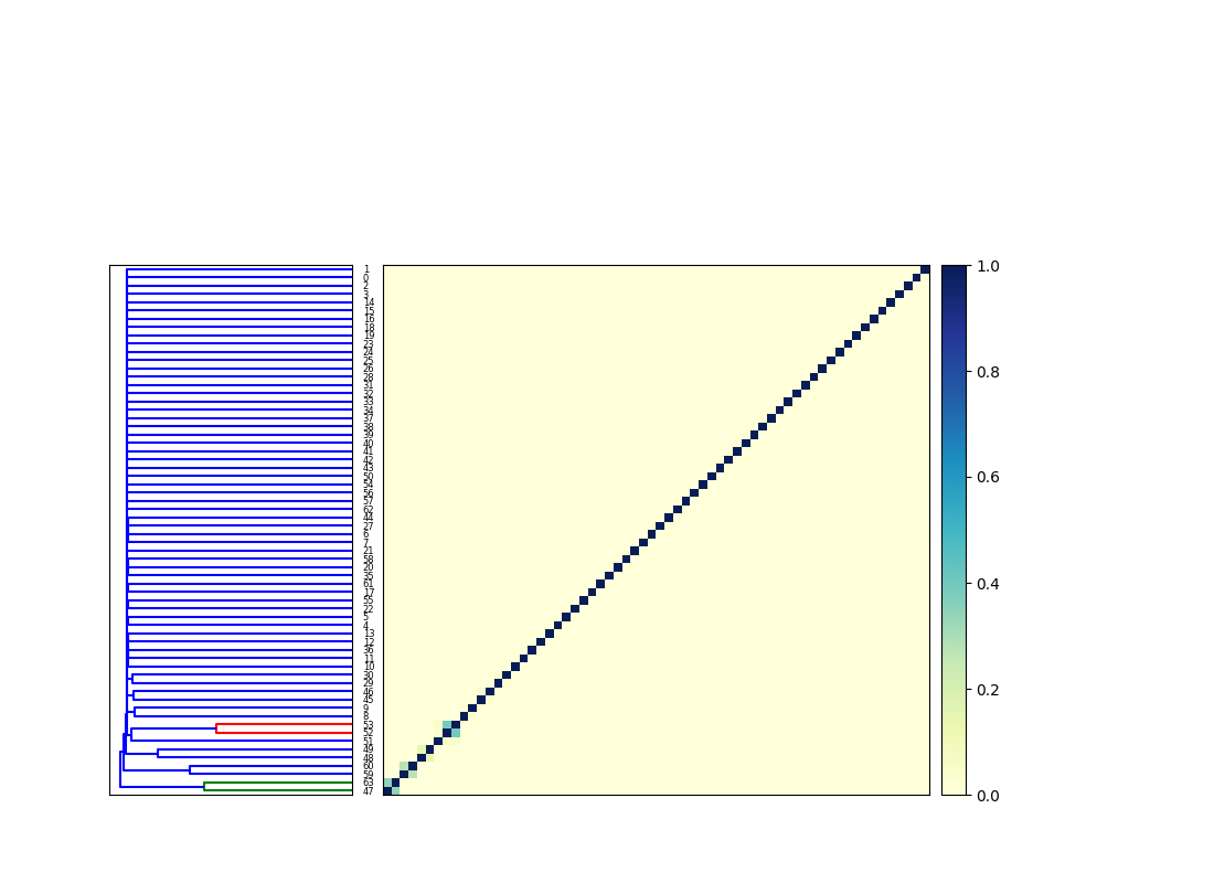
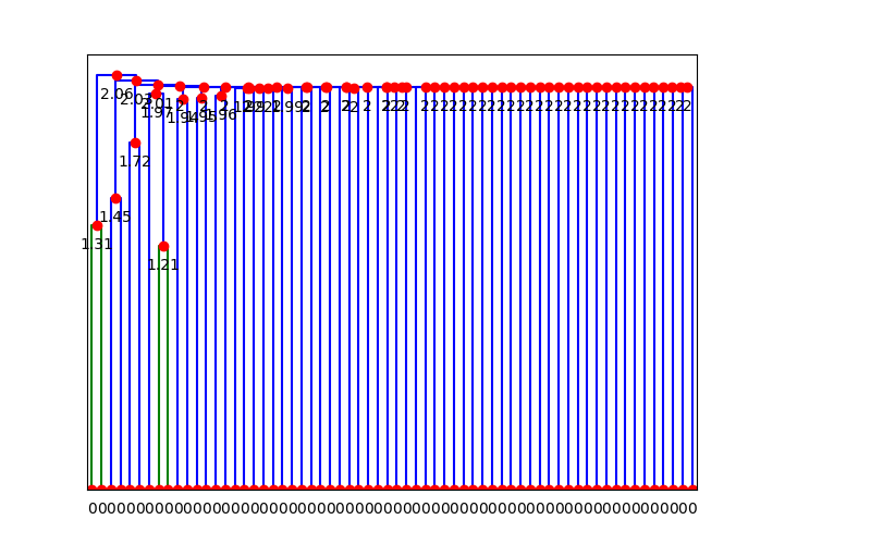
The dendrogram is then cut at some given phenetic distance - in this case I chose 1.8, based on visual inspection of this next dendrogram:
The cocluster.py script then outputs a cluster details CSV file that lists all of the clusters and their members. (The clustered signatures themselves are also provided, along with singletons.)
And, finally, all of this activity is logged and summarized in the results output:
...
total clusters: 60
num 1:1 pairs: 56
num singletons in first: 0
num singletons in second: 0
num multi-sig clusters w/only first: 0
num multi-sig clusters w/only second: 0
num multi-sig clusters mixed: 4
The full set of commands is listed in this Snakefile, and commands to repeat it are in the appendix below.
Playing with real data
Since both the Tully et al. and the Delmont et al. papers have been published now, I first re-downloaded the published data and calculated all the signatures for the 3500 or so genomes -- see the instructions and Snakefile in github.com/ctb/2019-tara-binning2/.
Once downloaded, computing the signatures takes about 15 minutes, using
snakemake -j 16.
Then, I ran the cocluster script from https://github.com/ctb/2017-sourmash-cluster like so:
./2017-sourmash-cluster/cocluster.py --threshold=50000 -k 31 \
    --first ../data/tara/tara-tully/*.sig \
    --second ../data/tara/tara-delmont/NON_REDUNDANT_MAGs/*.sig \
    --prefix=tara.coclust --cut-point=1.0
This took about 2 minutes to run on my HPC cluster, and produced the following output with a cut point of 1.0 (which is pretty liberal).
...
total clusters: 2838
num 1:1 pairs: 331
num singletons in first: 1886
num singletons in second: 443
num multi-sig clusters w/only first: 42
num multi-sig clusters w/only second: 4
num multi-sig clusters mixed: 132
When I re-run it with a more stringent cut-point of 0.1, I get:
% ./2017-sourmash-cluster/cocluster.py --threshold=50000 -k 31 \
    --first ../data/tara/tara-tully/*.sig \
    --second ../data/tara/tara-delmont/NON_REDUNDANT_MAGs/*.sig \
    --prefix=tara.coclust --cut-point=0.1
...
total clusters: 3520
num 1:1 pairs: 43
num singletons in first: 2557
num singletons in second: 906
num multi-sig clusters w/only first: 6
num multi-sig clusters w/only second: 0
num multi-sig clusters mixed: 8
Basically this means that:
- when doing stringent clustering, there are 3520 different clusters;
- 43 of the clusters provide a 1-1 match between bins from the Delmont and Tully studies;
- 2557 of the Tully signatures don't cluster with anything else;
- 906 of the Delmont signatures don't cluster with anything else;
- there are 6 clusters that contain more than one Tully signature, and no Delmont signatures
- there are 0 clusters that contain more than one Delmont signatures, and no Tully signatures;
- 8 of the clusters have more than two signatures and contain at least one Tully and at least one Delmont signature.
I'll dig into some of these results in a separate blog post!
--titus
Appendix: repeating the podar analysis
This workflow will take about 1 minute to run, once the software is installed.
To repeat the analysis of 64 genomes above (see output), do the following.
# create a new conda environment w/python 3.7
conda create -y -c bioconda -p /tmp/podar-coclust \
    python=3.7.3 sourmash snakemake

# activate conda environment
conda activate /tmp/podar-coclust

# grab the cocluster script and podar workflow
git clone https://github.com/ctb/2017-sourmash-cluster/
cd 2017-sourmash-cluster/podar-coclust

# clean out the existing files & run!
snakemake clean
snakemake -j 4 -p all
This last step will download the necessary files, compute the signatures, and run cocluster.py.
Comments !